
Back to Aerodynamic Design of Aircraft with Computational Software
Back to overview: Preamble Exercises and Projects
Chapter 7[pdf]:
7.1 Introduction
7.2 Zonal approach: Physical Observations
7.3 Mses - Fast Airfoil Analysis and Design System
7.4 Outer Euler Flow Solver
7.5 Boundary Layer and Integral Boundary Layer Models
7.6 Drag Calculation
7.7 Newton Solution Method
7.8 Airfoil Computations 7.9 Mses Design Application
Tutorial: MMs hands-on prep for MSES lab & HW
Exercises and Projects – software here MSES
The software is installed in the VM ToolKit. .../Ch7lab holds also octave scripts which run a specific workflow: Modify a given airfoil by scaling it for thickness and mapping the x-axis for crest movement. The run mesh generation, a single MSES run, and finally a Mach-sweep. An octave script plots results of all performed runs. You are advised to save already analyzed runs – clean up the directory – lest the plots become too cluttered. More detailed instructions are found in .../Ch7/Ch7Docs.
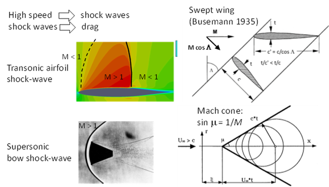
Background: Shock waves, the transonic airfoil problem and the blunt body problem
Fig. 1 summarizes some basics about shocked flow. The figure is repeated in Ch 9 for easy reference.
Review questions to consider before running calculations.
- Explain the domain decomposition idea used in MSES, based on Prandtl’s boundary layer hypothesis.
- MSES manages to compute also cases with small recirculation regions where the boundary layer flow is reversed and u = 0 at separation and re-attachment points. Look up the boundary layer PDE in Ch 2 and explain what problems they would encounter. How has MSES solved this problem?
- Explain how the Newton scheme enables also incorporation of global variables like angle of attack, lift coefficient, as constraints or degrees of freedom.
- The Newton scheme for the steady equations avoid the CFL limitations of explicit time marching scheme. But Newton requires a sufficiently good initial guess. How is this produced in MSES when it is used to compute a sweep of Mach-numbers. Look in the MSES manual (in .../Ch7/Ch7Docs) to see how the initial guess is produce for the first of the calculations in a sweep.
- MSES, like all CFD codes, will not compute all cases. Give two different reasons for an MSES to fail to converge.
- For incompressible, inviscid, flow the Bernoulli equation
p + q = const., q = dynamic pressure = 1/2 ρ u2
holds along a streamline.
The pressure coefficient is defined as
Cp = (p – pinfty)/qinfty,
where pinfty and qinfty are the static and dynamic pressures in the free stream far away from airfoil. Look up the definition of stagnation point and compute the value of Cp at a stagnation point.
- EXTRA: Compute Cp at a stagnation point in isentropic compressible flow given the flow Mach-number Minfty:
H = γ/(γ-1) p/ρ + 1/2 u2 = γ/(γ-1) pinfty/ρ_+ 1/2 uinfty2 (total enthalpy)
p = pinfty (ρ/ρinfty)γ
Airfoil computations with MSES
- In the VM directory .../raemod the “original” airfoil is the RAE 104. It is used as a baseline for modifications. Run the original RAE104 airfoil by the command
..>./runmses … note the ./ ! runmses is a command file in this directory, not a globally accessible command.
Change α to 3 deg in the MSES control file mses.raemod, then change M in that file and run M 0.5, 0.6, 0.7, 0.75. After a run, use the mplot program,
..> mplot raemod(mplotis a globally accessible command, likemset,mses, andmpolar)
make a Cp-plot by choosing first 1 and then 2. Check the MSES manual for options. Make a screenshot of the plots and save for your report. You may want to make more runs with M between 0.5 and 0.8 to answer:
What is Mcrit for this case?
(Hint: the mplot plot shows a dashed line for Cp*, the pressure coefficient at M = 1.)
What happens with the shockwave when M increases?
- Change
mses.raemodto the original, M = 0.5 and a 0.
Run ./runmses and then ./runmpolarmach.
Run octave modifyrae.m and change the thickness to 5% and 15% and re-run:
..>./runmses..>./runmpolarmach
Run octave plotall.m to produce a plot with CD(Mach) for the three foils. A rule of thumb says that drag varies with thickness squared. Is this consistent with the computed data?
The conclusion is that drag is very sensitive to thickness and the computations show this also quantitatively.
- Finally, go back to thickness 10% but move the max. thickness in the range fore -25% to aft +25%. Repeat the
modifyraeetc. runs for some selected crest movements. Can you find a crest position with better Mdd?
Compile the plots and explain your conclusions about transonic airfoil design:
Why can’t wings be so thin? Crest movement is a way to influence drag rise without changing thickness. Summarize your findings about this effort – easy?
- The Eppler387 airfoil is found as blade.eppler in the VM directory /Eppler together with an
mses.epplerandspec.epplerfile. The latter are set for M 0.5, α 0, Re 107 and an a-sweep. The Eppler foil is designed for low Re and Mach. Change to numbers reasonable for a glider of your choice at sea-level. Run the α-sweep to produce the drag polar table (it will bepolar.epplerunless you have decided to change it). It is quite probable that mses will experience problems with M < 0.1. Change to running msis and mpolis instead. These codes are for homentropic flow and the algebraic isentropy relation replaces the energy equation.
- Then run msis at increasing angles of attack and use mplot to see the development and movement of the laminar separation bubble.