
Back to Aerodynamic Design of Aircraft with Computational Software
Back to overview: Preamble Exercises and Projects
Chapter 5[pdf]:
5.1 Introduction and Overview
5.2 Curve and Surface Geometry Representation
5.3 Airfoils and Surfaces
5.4 Grid Generation
5.5 Sumo Mesh Generation
5.6 Euler Volume Grids by TetGen
Tutorial: MMs hands-on prep video for sumo
Exercises and Projects – software here SUMO
Review questions
- Explain the features of structured and unstructured grids of relevance for automatic meshing and solver complexity.
- Draw a sketch of a 2D quadrilateral finite volume grid and proper labeling for a) a cell-center version and b) a cell-vertex version.
- Draw a sketch of a 2D triangular primal grid with proper labeling and its median-dual grid. Don’t make the primal grid regular ! What shape will the dual cells have if the primal grid is structured rectangular ?
- Octave provides a Delaunay triangulation function. It produces the Delaunay triangulation of the convex hull of a set of points. Discuss how this could be used for mesh generation also of non-convex areas.
- Describe two common shape definition schemes, the CST scheme and the Bézier scheme.
Airfoil geometry calculations
- The script
CSTapprox.mcomputes the best CST representation of an airfoil scaled to x in [0,1], given as a set of points (xj,yj) on the curve (x(t),y(t)) with the parameter t chosen so
x(0) = y(0) = 0, and dx/dt (0) = 0
It treats the upper surface and lower surface separately. Say we get
yu = sqrt(x) sum(aj xj) = sum(aj x j+1/2), j = 0,...
a) Compute its slope and curvature at x = 0 of yu(x). The lower surface is
yl = sum(bj x j+1/2), j = 0,...
What is the condition that the combined curve has curvature continuity at x = 0?
The problem can be formulated as a linear least squares approximation problem:
              min over {aj}, j = 0,1,..,n
              sum(yu(xk) – yk)2  yu(x) = sqrt(x)(1-x)sum(aj xj)                 (1)
b) Show that the limit as t -> 0 of y(t)/sqrt(x(t)) is C sqrt(2R) where R is the radius of curvature at x = 0. What is the constant C? This means that the data will not explode close to t = 0.
A few airfoil files are given as foilname.dat, for example .../Ch5/goe298.dat. Many more are found in .../Ch5/Airfoilfiles.
c) The CSTapprox script reads the file, interpolates a cubic parametric spline, evaluates that at many points and then computes and plots the curvature. It goes on to compute the CST representation of your chosen degree n, plots it and its curvature, and reports the RMS and Max errors erms(n) and emax(n) from (1). Run with successively increased n. Why does the error suddenly drop to 0 when the degree is increased? Is the CST foil useful at that degree?
Geometry modification with sumo
The following labs all use the sumo simplest default model, the winged cigar ellipsoid body with a main wing. sumo is controlled best with a mouse with scroll wheel; touch pads seem not to work well for right clicks.
- Experiment with the rotation parameters for the wing: right-click the wing in the geometry tree in the left pane and choose to edit it. sumo performs the rotations in the sequence x, y, z. Try Rx = 90o and Ry 90o. Find another set of rotations to give the same effect.
- Sweep the wing leading edge 45o, keeping the sections parallel to xz-plane and the span constant. This requires you to figure out the new (x,y,z) of the tip leading edge. Click the wing in the component tree to show the sections, right-click the tip section to edit it and change the coordinates. Note the port wing is a mirror copy of the starboard wing.
The VM toolkit ceasiompy environment provides the cpacscreator for interactive editing of aircraft geometry stored in the CPACS XML format. Such a file can be sent to sumo for automatic Euler meshing.
Surface and volume mesh generation with sumo
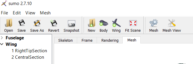
Generated surface meshes are shown by sumo in the Mesh view. The volume mesh can be inspected with the dwfscope companion module to sumo.
The task is to generate the default volume mesh for the winged cigar and inspect it.
Click on the Mesh icon, then the create mesh button, OR pull down the Mesh menu and choose create mesh. When finished it puts up a window with surface mesh statistics. Click its Volume mesh button, which brings up the Generate Volume Mesh window, click run to generate the volume mesh with default parameters. The window will say tetgen terminated normally and show mesh statistics. Save the volume mesh in sumo standard format: Pull down the Mesh menu and choose Save Volume Mesh, give it a name of your choice. Then start dwfscope:
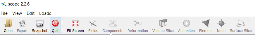
click the Open button and select the .zml file you just generated. You see the surface mesh. To see sections of the tetrahedral mesh, click the Volume Slice icon, select the type of plane (say, xz plane offset by 1) and click apply. Zoom in by scroll-wheeling, rotate around center of view by left-button mouse movement, and around a far away center, much like panning, by right-button mouse movement.
Pull down View menu and choose Mesh quality display. Clicking Show will show badly shaped tetrahedra in contrast color. In this experiment, there were 13 offending tets:
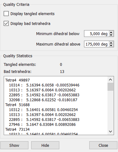
The Delaunay algorithm needs to break ties when two or more possible actions seem equally good, and does this by random choice, so the results of another experiment may be different. Bad tetrahedra with small volume (needles or slivers) will not hurt the inviscid finite volume solver. But bad elements in RANS boundary layers are to be avoided. The Pentagrow boundary layer mesh generator called “Hybrid” in the sumo Generate Volume Mesh window makes pentahedra close to the solid surfaces: These can be “tangled” and do harm a RANS computation.
Now is the time to explore the parameters in the Generate Mesh surface mesh, and in the Generate Volume Mesh volume mesh control windows on the isotropic meshes suitable for inviscid flow solution. Consult the sumo mini-manual (pdf in .../Ch5Docs) for explanations.