Back to Aerodynamic Design of Aircraft with Computational Software
Back to overview: Preamble Exercises and Projects

Chapter 3[pdf]:
3.1 Introduction - Mapping Planform to Lift and Drag
3.2 Computational Vortex-Lattice Methods
3.3 Planform Design Studies with VLM
3.4 Wings for High Speed

Tutorial: —

Review questions

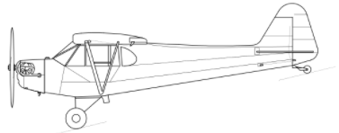
1. Look at the Biot-Savart equation (3.5). Where does it produces infinite velocities? Consider now a VLM model with a symmetric main wing ahead of a vertical tail in the symmetry plane and a horizontal stabilizer. The model assumes that the trailing vortices follow free stream streamlines. Consider the Piper Cub J-3 in the sketch below, from Wikipedia. Sketch in the angles of attack where we expect trouble from trailing vortices hitting collocation points or bound vortex midpoints. Yet the Cub flies just fine. Discuss the effect of the fuselage. In zero sideslip, the wing horseshoe trailing leg in the symmetry plane should not create problems in the force calculation anyway. Why?

2. Assume that a pair of wingtip vortices Gand -G, separated by wing span b (actually, they will converge somewhat from the wing tips) are infinitely long and horizontal. How fast do they sink – or rise? Using the simplest constant-strength Prandtl lifting line model, compute G for a Boeing 747 at take-off weight around 350 metric tons. You will need more data, easily available. Constant strength is wrong; re-do the calculation assuming elliptic lift distribution; that model sheds a variable-strength wake. Assume that it rolls up so all vorticity from the right half is concentrated to the wing tip trailing streamline. What is its strength?

VLM computations

The script tor1.m computes a quadrilateral wing defined by AR, taper ratio ct/cr , quarter-chord sweep angle Sweep, dihedral Dihed, and Twist for some airspeed, altitude, and angle of attack a. It produces a row in a table of the parameters (angles in radians)

     AR   ct/cr   Sweep   Dihed. Twist   alpha 

and a corresponding row in a table of the force and moment coefficients

         CL    CD    CY    Cl    Cm    Cn

tor1(AR,tap,swe,dih,twi,alt,airspeed,alpha,foil1,foil2,resimn,resimx)
resimn and resimx define refinements of the initial paneling:                       
         nx = 2^(res-1) nx0 for res = resimn… resimx.
so resimn = 2 and resimn = 4 runs original, doubled, and quadrupled paneling used to extrapolate the results, in VLM_e.m described below.

3. Check how the VLM estimates for C_L, C_m converge with the number of vortices. Run with script tor1.m an AR 8 rectangular wing with symmetric profile and
                 Nx = 2^k, k = 1,….. and Ny = 4Nx, a = 5 deg.
   Use resimn = resimx = 2,3,4,5. Plot C_L, C_m and C_D vs. 1/Nx. Theory shows that 
                 C_L(1/Nx) = C_L(0) + C1/Nx + smaller terms.
   This allows extrapolation to Nx = Infty:  
                 C_L(0) = 2 C_L(1/(2Nx)) – C_L(1/Nx)
   is usually a better approximation than even C_L(1/(4Nx)) and much cheaper since the work grows like Nx⁴. The extrapolation can be continued with results from 4 Nx, 8 Nx, … (but 8 Nx costs 4000 x the compute time of Nx). Systematic mesh refinement with at least three levels is a due diligence check that the convergence follows the theory so bad results from under-resolution, ill-conditioning, or “close encounters” can be spotted. The function VLM_e.m performs calculations of force and moment coefficients for a sequence of refinements of a user-defined initial coarse paneling.

4. Then try a straight wing with AR 2, 4, 6, 8, 10. Run an alpha sweep withtor1.m and check dC_L/da (small a) vs. the formula in Ch 3.  The script ARsweep.m runs a list of AR and a using tor1.m which in turn uses VLM_e.m and produces tables partab and restab with rows described above. Your job is to compute C_L,a from the table.

5. The script tor1.m computes a quadrilateral wing with sweep, taper, and twist. Your job is to experiment with sweep and taper for an untwisted wing. Modify ARsweep.m to make an (AR, taper, a) sweep and fit
                 C_Di = C_D0i + k C_L²
   to the computed points for each (AR,taper). The wing (induced drag) efficiency factor is e = k/(p AR) where lifting line theory predicts that  e_max= 1 for an elliptical flat wing.
   Fix AR at 6.  Then run a quadrilateral tapered wing with  ct/cr = [0.3, 0.7, 1] and quarter-chord sweeps [0,30,60]^o. Note the e and C_D0i so computed as well as C_L,a. Before analyzing the data, add a rough estimate of C_D0,viscous of 150 cts to C_D0i. Show that the best L/D (which determines best glide slope) is LoD_max = 1/sqrt(k C_D0tot). Which wing has best glide slope?

6. The file GAV.m has a Tornado model for a Piper Cub-like generic general aviation airplane and its weight and CG-location. What angle of attack and elevator angle will trim it for straight and level flight at sea level and TAS 35 m/s? Suppose C_D0v = 0.0150. What thrust is required? First, neglect the elevator influence on lift to find a, then for this a find the correct elevator angle ele. A more accurate procedure is to assume “linear aerodynamics”. Compute the derivatives C_L,a , C_m,a, C_L,ele and C_m,ele  from a computed table produced by (a,ele)-sweep and solve the linear system 

             qS(0 + α CL,α + ele CL,ele) = W,
             qScMAC (0 + α Cm,α + ele Cm,ele) = 0