
Back to Aerodynamic Design of Aircraft with Computational Software
Back to overview: Preamble Exercises and Projects
Chapter 10[pdf]:
10.1 Introduction
10.2 Stability of Aircraft Motion
10.3 Flight Simulation for Design Assessment
10.4 Building Aerodynamic Tables
10.5 Applications Configuration Design and Flying Qualities
Tutorial: Under construction.
Exercises and Projects – software here VLM, SU2
Review questions to consider before doing calculations
- Explain why the CG must be ahead of the aerodynamic center for longitudinal stick-fixed stability. Give the definitions of the italicized terms.
- What is tip stall? Why is it to be avoided, especially on swept wings?
- The TCR computed below has, like the Concorde and many other high-speed craft, a highly swept inner wing leading edge. Thinking of low speed flight, what does it contribute? Can VLM model that?
Configuration computations
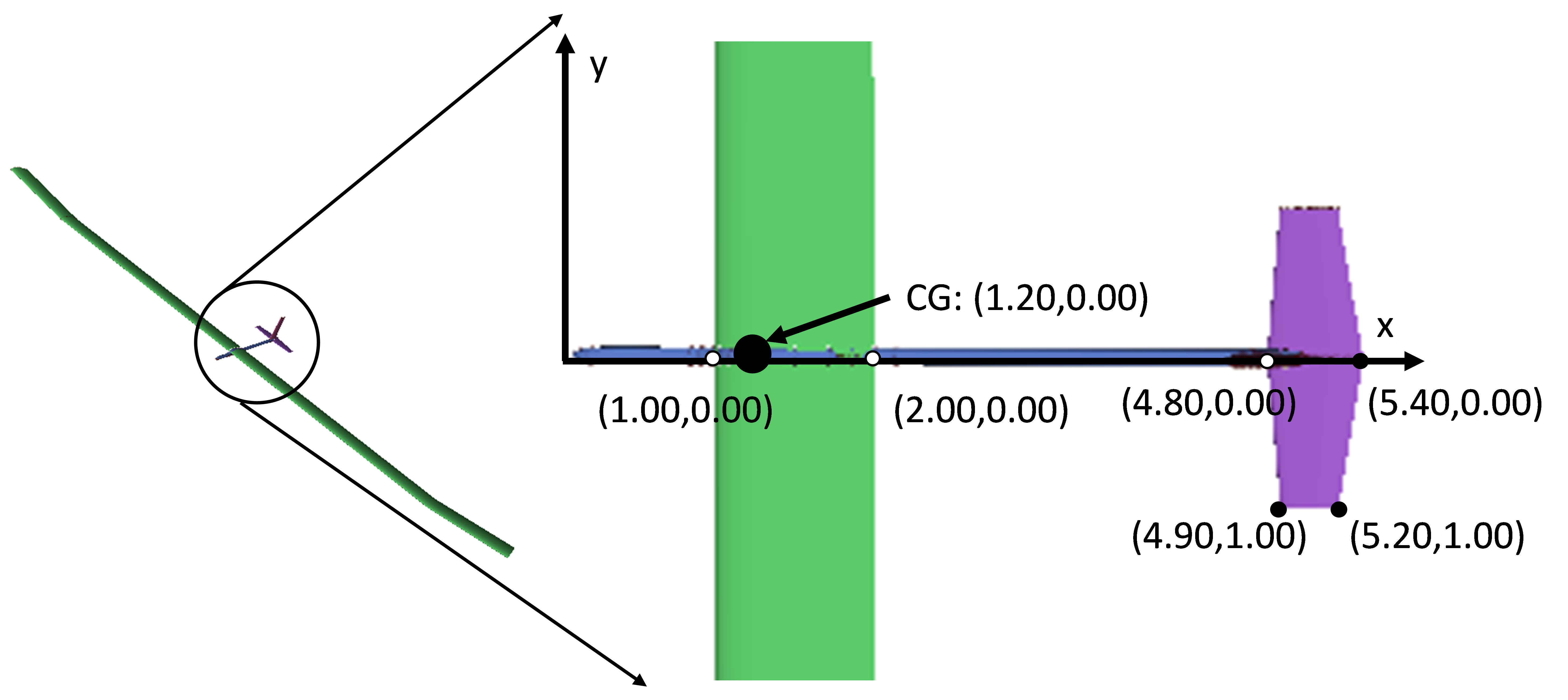
- A balsa glider model. Proper flight simulation needs mass, CG location, and mass moments of inertia. The file glider.BMP shows the scan of a balsa glider toy made from balsa sheet. balsa.txt holds the 3D coordinates of the outlines of the body and lifting surfaces in assembled form. The script
read_plot_balsa.mreads the file and plots the outline of the polygons. The body is 3 mm and the lifting surfaces 1.5 mm thick. The units are m and the density of the balsawood is assumed to be 160 kg/m3. Your job is to compute the mass, CG and mass moments of inertia of the assembled model. The function
[iner,area,cg] = weibalpoly(xyz)
computes inertia tensor iner around its CG, area area, and CG cg of a constant thickness plane surface bounded by the vertices in xyz. Add up the contributions Volj, CGj, and Ij from the fuselages and wings:
              Vol = sum(Volj);
              CG = sum(Volj  CGj)/Vol
              I     = sum {Ij + Volj [|CGj - CG|2 – (CGj-CG)(CGj-CG)T]}  ... (3)
((3) is the “parallel axis theorem” of rigid body mechanics, look it up if unsure). Vectors are column vectors. There is a lead weight at the nose. What must it weigh to give pitch static margin 10% of main wing chord? You may assume that AC is at wing quarterchord.
- Compute the longitudinal stability margin at M 0.5 on the TCR by VLM. A sumo file TCR15.smx and a VLM geometry definition file TCR15.geo produced from it are provided. An octave script geo2table.m uses the
VLM_e.mfunction to write a table (see Ch 3 exercises) of flight state parameters (Mach, alpha, beta, …) and force and moment coefficients.
- HALEbook.smx and HALEbook.geo describe a typical High Altitude, Long Endurance configuration with no details of propulsion, fig. 1 below. Google the Airbus Zephyr to see an IRL example. Use the volume coefficient (see Ch. 10) to size the existing placeholder horizontal tail. The horizontal tail is all-moving around its quarter-chord line. The wing span is 30 (!) m,
Compute dCm/dele from CL,α = 2p/(1+2/AR), flat plate AC = 1/4c, the tail arm to CG, and other data given in the figure. Compare with dCm/dele obtained from VLM computations. Suggest aerodynamic reasons for the differences.
- Use the HALE model and an alpha-sweep to compute the longitudinal stability margin. What alpha is required to stay aloft at M 0.1 at alt. 20000 m if the mass is 80 kg? Run a beta-sweep at that alpha, suggest a stability requirement for sideslip and define and compute a quantity for sideslip analogous to the longitudinal static margin.
- Run ModelIA swept wing (see Ch 6 Exercises) with SU2 in inviscid mode with an M sweep from 0.5 to 1.1. Neglect the necessary elevator deflection to balance the moment, choose a(M) to give constant lift (not lift coefficient) across the M-range. Explain why α M2 is expected to be approx. constant and select α = 2 deg at M 0.5. Check that the computation bears out the expectation.
- Vortex lift on highly swept wings at high angle of attack is not modeled by our VLM code. The leading edge suction analogy empiricism by E. Polhamus was incorporated in e.g. the VORSTAB NASA VLM code from the eighties. We recommend instead to go up the fidelity scale and use SU2 Euler. To this end, delta60.smx and delta60.geo are provided, modeling a 60o swept delta wing with quite sharp leading edge. Run an alpha-sweep up to 15o with SU2 and VLM and plot the lift curves so obtained. The sharpness of the leading edge is essential for make the inviscid flow separate on the leading edge. But the exact separation pattern can be obtained only by RANS.