
Back to Aerodynamic Design of Aircraft with Computational Software
Back to overview: Preamble Exercises and Projects
Chapter 1[pdf]:
1.1 Introduction
1.2 Advanced Wing Design - Cycle 2
1.3 Integrated Aircraft Design and MDO
1.4 Aerodynamic Design and CFD
Review questions
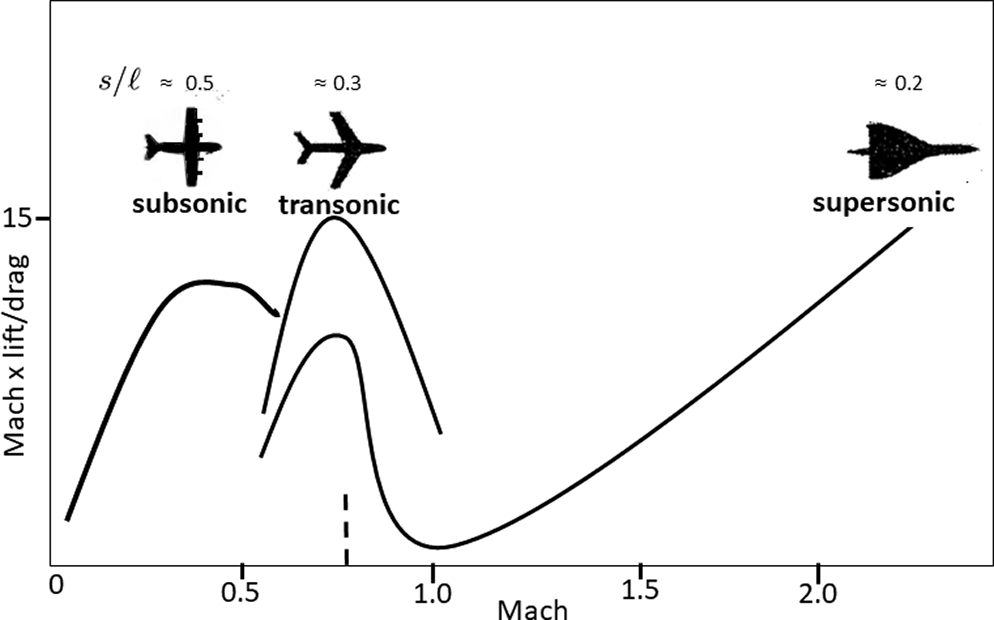
- Explain why the subsonic planform L/D curve in Figure 1.14 (reproduced below for easy reference) falls off with increasing Mach.
- Explain/justify the idea of weakly coupled MDO
- Give and explain examples of CFD data exchange with other disciplines
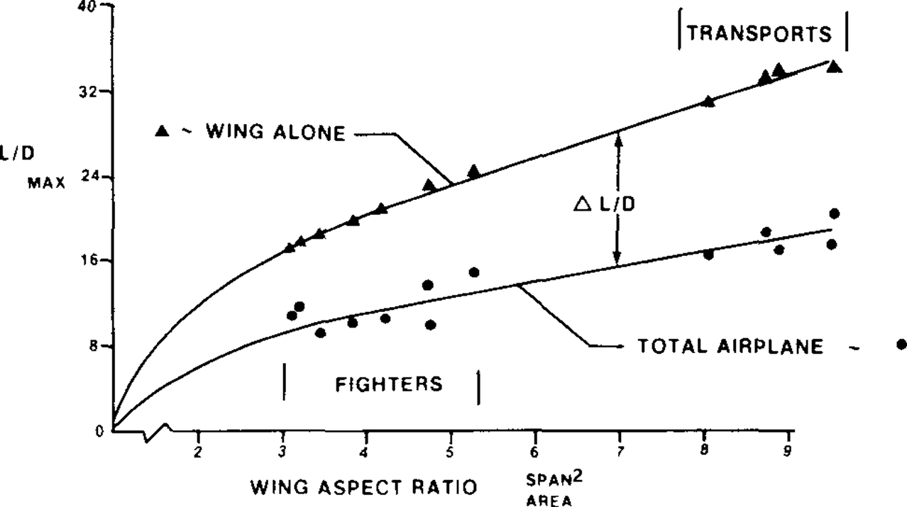
- Fig. 1.3 (reproduced here for easy reference) shows how L/D max varies with AR. Use the approximate relation Eq. 1.5

to check the shape of the curves.
- Show on a finite – dimensional optimization task,
              min g(y), y = (flow) variable dim N
              s.t. f(x,y) = 0, x = shape parameters of dim M, M << N
why the computation of dg/dx by adjoint costs 1/M of use of direct gradient (some more text on website is promised in book)
Hint: dg/dx = dg/dy dy/dx; df/dx + df/dy dy/dx = 0, so direct gradient
dy/dx = – (df/dy)-1 df/dx
df/dy is NxN matrix, dy/dx and df/dx are NxM and dg/dy is 1 x N.
So,
dg/dx = – dg/dy (df/dy)-1 dy/dx.
How should this matrix product be computed?
- Here are relevant data for a Piper J-3 Cub and sea-level atmosphere

b = 10.74 m, MTOW = 550 kg, S = 16.6 m2, ρair = 1.2 kg/m3.
Best Rate of Climb (Vy) 450 ft./min, Absolute Ceiling 14,000 ft., Cruise Speed 73 mph,
Top Speed 83 mph, Stall Speed (Vs) 39 mph, Best Glide (Vgl) 50 mph
Drag polars for the Piper may be available, but we can use the data above to find an approximation
CD = CD0 + k CL2
which is quite good; thus, k and CD0 are to be found. First, lifting line theory gives an estimate for k,
k = 1/(e π AR)
where e is the span load efficiency, its maximum is 1 and it will be taken as 0.85.
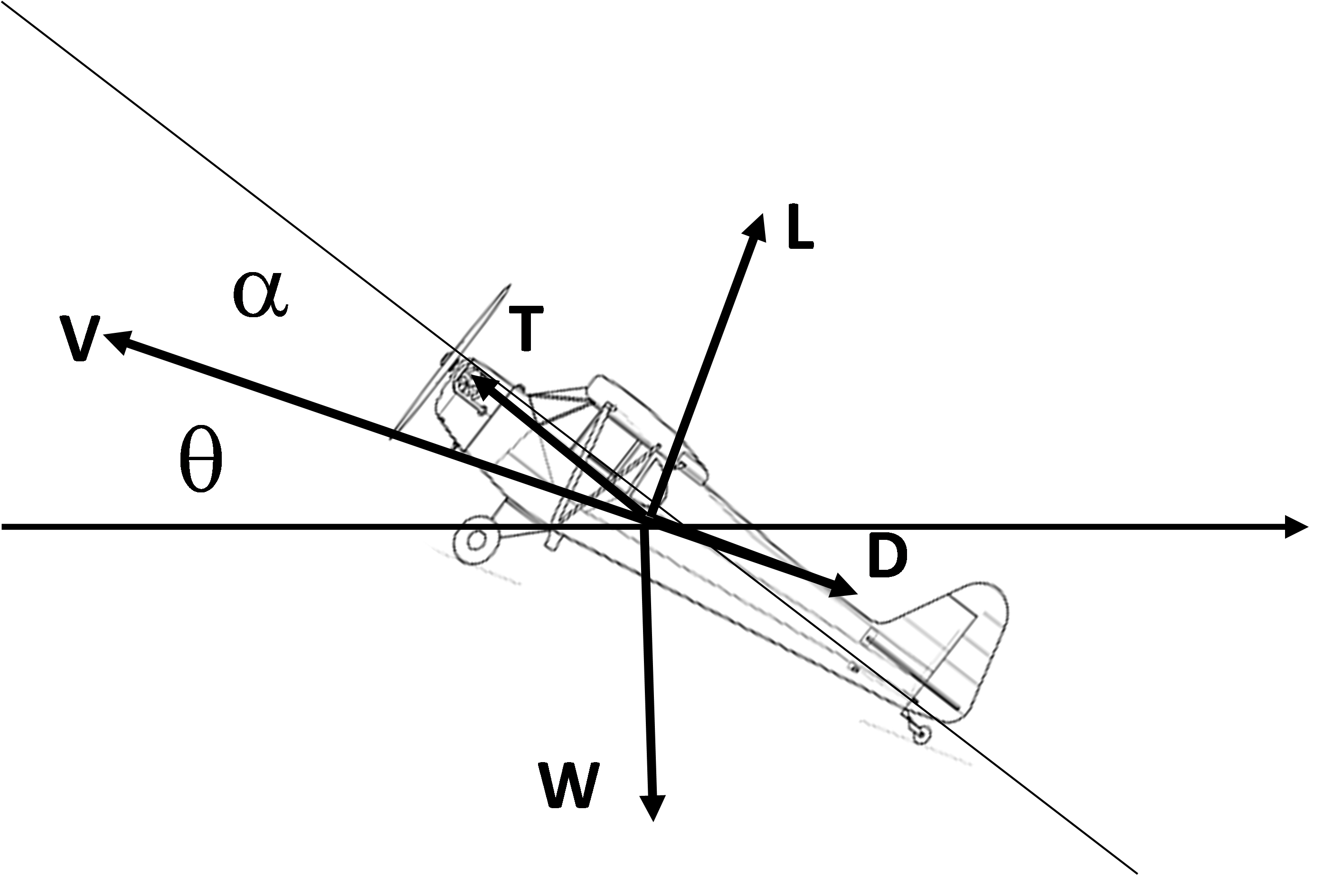
The equilibrium equations with angle of attack α and flight trajectory angle q, assuming thrust vector aligned with aircraft waterline, are
T sin α + L – W cos α = 0 (1)
T cos α – D – W sin α = 0 (2)
In a glide T = 0. Show from the ratio of (1) and (2) that the best glide angle has
θopt = – atan(1/max(CL(α)/CD(α)) = – atan(sqrt(k CD0)) approx = – sqrt(k CD0) ,
CDopt = 2 CD0
Use this in (2) to conclude that
CD0 = [W sqrt(k) / (ρair S Vgl2)]2
The numbers so produced have been used in the tables in the cfd.m function to be used in the exercises to follow.
- Actually, W and S should be considered design parameters.
For straight and level flight, θ = 0, there are four variables: T/W, W/S, a and V, constrained by two relations
T/W W/S cos α -1/2 ρair V2 CD(α) = 0
T/W W/S sin α + 1/2 ρair V2 CL(α) – W/S = 0
This is the classical situation illustrated by carpet diagrams. Rename W/S x and T/W y:
x y cos α -1/2 ρair V2 CD(α) = 0
x y sin α + 1/2 ρair V2 CL(α) – x = 0
Plot a T/W (y) vs. W/S (x) -diagram for sea-level flight as follows:
make lists Vlist(1:nV) and alist(1:na)
for i = 1:nVfor j = 1:na% solve equations for x and y to get x(i,j) and y(i,j)end j% plot the curve {x(i,:),y(i,:)} end i for j = 1:na% plot the curve {x(:,j),y(:,j)} end j
The diagram shows that: It is possible to fly with some given thrust and weight for two different (α, V), one with high α and slow V, the other faster with lower α. These coincide at the lowest thrust possible to stay aloft. Suppose you fly at best cruise. What happens if you increase α? Throttle up without changing α?
- The folder .../Ch1 has routines for running a non-linear optimization problem with the Octave
fminconoptimizer from theoptimtoolbox.fminconsolves a problem defined by an objective functionobjf(X), lower and upper bounds lb and ub on the parameters X, and non-linear constraints – equality and inequality – defined by the function constr(X). Theopt1.mscript runs the optimization; select the problem by setting the global variable DEMO to 1 or 2.
DEMO = 1 considers the problem to find the angle of attack a and airspeed V for minimal thrust in straight and level (θ = 0) sea-level flight – best cruise.
              min over (α,V)   T =  D/cos α=  q S CD/cos α
              q = 1/2 ρair V2
              subject to the constraint
              L = q S CL >=  W,  - T sin α = W - q S CD tan α .
Since W = MTOW g , S, and ρair are constant, we can scale the problem.
Let r = 1/2 S ρair, w0 = W/r;
find
              min   V2 CD(α)/cos α over X = (α,V)
              subject to the constraint
              V2 CL(α) >=  w0  - V2 CD(α) tan α
The aerodynamics is defined by the CL(α), CD(α) tables so the cfd function just interpolates in the tables and returns [CL CD].objf calls on cfd to get prop, and returns FoM. constr calls on cfd to get prop and returns c which must be <= 0.
The demo program opt1.m solves this problem.
- Run the program with different wing areas (different wing loadings) and note the optimal α.
- Verify the observation by analytically showing that the optimum occurs for the α which maximizes CL/CD + tan α – which if these terms dominates ?
- Then show that L/D max is easily found as the point where a line through the origin is tangent to the drag polar.
- How do your results compare to the cruise speed given in Exercise 6?
The next task is to modify the objf and constr functions to find the α,V,θ,T which maximize climb rate
V sin θ when thrust is limited to Tmax. Let r = 1/2 S ρair, w0 = W/r
              max V sin θ over (α,V,θ,T)
              T cos α – V2 CD(α) – w0 sin θ = 0
              T sin α + V2 CL(α) – w0 cos θ = 0
              T <= Tmax/r
The problem is solved by setting DEMO = 2 in opt1, constr then defines two equality constraints, and the limit on T is an upper bound in ub. Your job is to fill in the missing lines of code and run the optimization with different starting guesses.