
Back to Aerodynamic Design of Aircraft with Computational Software
Back to overview: Preamble Exercises and Projects
Chapter 4 [pdf]:
4.1 Introduction to Computing Flow with Shock Waves
4.2 Finite-Volume Methodology
4.3 Time Integration Schemes
4.4 CFD WorkFlow for Nozzle Problem
Tutorial: ARs hands-on prep/lecture for DemoFlow
Exercises and Projects – software here DemoFlow nozzle & shocktube
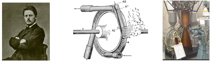
The Laval nozzle – converting pressure difference into speed to turn a turbine.
A “Laval” nozzle has a converging entry section with area going from inlet A0 down to A* – the throat – and a diverging section from A* to the exit A1. Rocket engines have similar designs. The task of the nozzle is to convert pressure and heat into speed, to turn a turbine wheel, or by momentum flow to push the rocket, Fig. 1.
The model simulated by the DEMOFLOW program is for inviscid, perfect gases. The realism is of course questionable, but its task is to acquaint the student with typical flow solver parameters for compressible flow CFD codes such as SU2. The simulation models everything upstream of the nozzle as a huge reservoir with given pressure p01 and temperature T01 and d:o downstream where only p2 needs be specified. The first tasks here are to review the features (misfeatures?) of the model
Review questions to consider before experimenting with the program
Basics of the model:
- The code is for choked nozzles with sonic flow at the throat. With p2 = p01 there is no flow. But blowing gently through a nozzle is certainly possible without reaching Mach 1 at the throat. Assume steady, incompressible flow and apply the Bernoulli relation to estimate the ratio A1/A* at which the throat becomes sonic, M = u/a = 1. The use of correct compressible, isentropic flow relations is much more complicated. Here they are, for easy reference:
       Entropy:          p/p01 = (ρ/ρ01)γ;
       Perfect gas:      p = RρT, R = gas constant for air (J/kg, K),
                         R = cp – cv = (γ - 1)cv, γ = 7/5,
                         a = sqrt(γ p/ρ)
       Total enthalpy:   γ/(γ-1)p/ρ + 1/2 u2 = γ/(γ-1)p01/γ01;
       Mass flow:        ρ u A(x) = const. = q
- The quasi-1D formulation neglects the transversal velocity components. Consider a streamline along the curved wall in the divergent part and apply the streamline curvature equation in exercise 2.8. What does that say about pressure difference between throat and exit for incompressible flow?
- The figures below show Schlieren pictures of outflows from a nozzle and M and p/p01-sketches through the nozzle for different values of p01/p2. A Schlieren picture shows density variations.
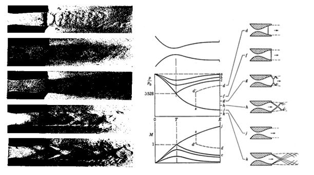
What does that imply about the realism of the downstream conditions? The choked flow with a shock in the nozzle is at the top. The downstream pressure is reduced as we go down. Why no pictures of the isentropic, subsonic cases?
Numerics
- Why are the unsteady equations used even when we look for a steady solution?
- There are two time stepping schemes, ‘implicit’ and ‘explicit’. Explain the meanings of the terms, and describe the basic differences between them. Which takes less computing to perform a time step? How can an implicit scheme still be faster to reach a steady state?
- A theoretical estimate says that the solution will steady in about T time units. The flow model is inviscid so there is no damping as such in it. What mechanism dissipates the “energy” in the initial “error” ?.
Show that the computation needed to reach steady state with an explicit scheme is proportional to the number of grid cells squared.
- The available spatial discretizations are the Jameson central scheme and the Roe High-Resolution scheme. Central schemes are prone to wiggles and overshoots at shocks. What parameters control this (mis)feature? What ingredient in the Hi-Res scheme aims to produce a total variation non-increasing solution? First define total variation of a function f(.) over the interval I.
- Explain the meaning of the terms CFL, dissipation and dispersion.
Problems requiring formula manipulations
- The outlet conditions for subsonic flow combine p2 with extrapolated values of the two Riemann variables w2 = u + 2c/(γ-1) and w1 = entropy S = p/ργ. Compute the primitive variables u, ρ, p, E from p2, w2 and w1. Repeat by deriving and using the linearized entropy condition γ ρ dp = p dρ ( dp = p2 – p, etc.)
- D:o, subsonic inflow conditions, from w0 = u – 2c/(γ-1), S = p/ργ = p01/ρ01γ, and total enthalpy H = γ/(γ-1)p/ρ +1/2u2 = γ/(γ-1)p01/ρ01
Having dealt with the basics we turn to
Numerical experiments
The idea is to run the program in what-if mode. Always try to predict what will happen BEFORE pushing the button. Immediate feed-back helps climbing the learning curve more quickly!
- First run the case set up as standard and observe the shock position. Choose to define the solution by the back pressure (radiobutton “States“). Note that the default defines the exact solution by setting the shock position; the downstream reservoir pressure is neglected.
- Then lower the exit pressure until the shock appears very close to the exit. What happens if you decrease the pressure further? And even further? Explain the behaviour by considering the outlet boundary conditions.
- Increase the back pressure until a subsonic solution appears. This requires a very small pressure difference. The code may take very long to converge! The solution plots show pressure waves bouncing back and forth between nozzle ends. It is obvious that they reflect with little energy leaked out. In fact, with such small velocities, the thermodynamics and kinematics interact weakly – the energy equation can be left out, and the model becomes linear – the wave equation. Better “non-reflecting” boundary conditions can be designed for such cases.
- Why are the back-and-forth sound wave reflections NOT so present in a choked nozzle with partially supersonic flow?
- Look at the pressure display. p01 is the upstream reservoir pressure. Why is the pressure at inflow NOT the same as the upstream reservoir pressure? Why is it possible to have a flow with inflow pressure LOWER than exit pressure?
- If you set inflow and outflow areas to 1 the code runs a shock-tube experiment with upstream conditions in half the tube. Run only a few timesteps of the explicit solvers, adjust the plotting frequency, increase the number of points, experiment with CFL. Fig. 4.x in the book shows results of first order Roe, Jameson, and Roe Hi-Res results. The Hi-Res result reported there uses the first order Runge-Kutta time stepping scheme which is not available through the GUI. The DEMOFLOW standard Runge-Kutta scheme adds temporal dissipation which smooths the otherwise sharp fronts of the Hi-Res scheme. Note that this does not add dissipation to the steady state, as discussed in the book section about semi-discretization.
Solver parameters
- The time step size is adjusted by changing the CFL number value for the Explicit solver. Run the Explicit Roe solver with all the default settings except:
Timesteps = 2000, CFL set to 1, then repeat with 2, then repeat with 4
It might be necessary to run the solver several times in a row for low CFL before reaching convergence. Convergence is signaled by the SOLVE-button text changing to Convergence.
Describe the convergence behavior in each of the three cases. Are they all stable?
Explain the reasons for this behavior. Does there seem to be an optimal size for CFL?
- Effect of the choice of the solver: Explicit vs Implicit
Run the Implicit Jameson solver with the default parameters except:
Timesteps = 50
Describe the convergence behavior. Is it stable?
Observe the timestep size variation (by clicking the ”Stepsize” button) and compare it to the timestep size in the Explicit Roe computations in 2.
Compare the time per iteration with the one of the Explicit Roe computation in 2. Explain the difference.
Observe the number of iterations and the time elapsed needed to converge and compare them with those for the Explicit Roe computations in 2. Explain the reasons for the differences.
State your conclusions about the trade-off between the number of time steps and the time taken per time step to reach steady state solution.
Observe and compare the residual history when running with the default parameters for Explicit Roe and Implicit Roe. State your conclusions about which solver to use when only a moderate residual is needed for the solution. And which solver is more efficient when a more accurate solution is needed ?
- Effect of artificial dissipation coefficients Vis2 and Vis4
Run the explicit Jameson solver with the default parameters except:
500 iterations, Vis2 set to 0.1 (and then repeat with 1, and then repeat with 2)
CFL = 1.5
What do you observe for the lowest value of Vis2?
State your conclusions about the effect of the artificial viscosity coefficient Vis2.
Then run again the explicit Jameson solver with the default parameters except:
Vis4 set to 0.02 (and then repeat with 0.04)
CFL = 2.15
State your conclusions about the effects of the artificial viscosity coefficient Vis4.