Back to Aerodynamic Design of Aircraft with Computational Software
Back to overview: Preamble Exercises and Projects
Chapter 2[pdf]:
2.1 Introduction to Wing Flow Physics
2.2 Shape determines Performance
2.3 Boundary layer development
2.4 Physics of Wing-Lift Creation
2.5 Behavior and Interaction of Flow Phenomena
2.6 Drag Taxonomy
2.7 Example: Swept-Wing Flow Physics
2.8 Physics Models - The Equations
2.9 Averaging for Turbulent Flows
Exercises and Projects
- The dimpled surface of a golf ball makes the flow turbulent. Fig. 2.13 visualizes the difference: the turbulent flow stays attached longer than the laminar flow, and the laminar flow separates with large coherent vortices. They create large-scale unsteady forces on the ball, making its flight more unpredictable. But the dimpled ball also flies farther. Why?
- An example of a non-intuitive aerodynamic device is the Gurney flap, invented by race car designer Dan Gurney. Look up the Wiki on Gurney flaps. First sketch your idea of the flow mean streamlines at the trailing edge, then find a publication with computed results to compare. Note that Gurney flap simulations are very expensive since they must employ unsteady flow models.
- Free stream Mach M and Reynolds number based on chord length Rec are two non-dimensional numbers which indicate compressibility and viscous effects, viz. It follows that a scale model experiment should reproduce both for the results – forces and moments – to be reliably predicted for full scale free flight.
For two different configurations, a high altitude autonomous craft with wing chord 1 m at altitude 20,000 m and TAS 35 m/s, and a transonic jetliner with wing chord 3 m at altitude 10,000 m and TAS 250 m/s, compute M and Rec and compute for a half-scale and a one-fifth scale model the sea level wind-tunnel speeds required to match M and Rec. An ISA (international standard atmosphere) table giving thermodynamic properties vs. altitude is reproduced here for easy reference. Look up “cryogenic” and “pressurized” wind tunnels and explain how they work. ρo = 1.2250 kg/m3
| Elevation z (m) | Temperature T (K) | Pressure p (bar) | Relative Density ρ/ρo | Kinematic Viscosity n x 10-5 (m2/s) | Thermal Conductivity k x 10-2 (W/m K) | Speed of Sound c (m/s) |
| 0 | 288.15 | 1.01325 | 1.0000 | 1.461 | 2.534 | 340.3 |
| 10000 | 223.3 | 0.2650 | 0.3376 | 3.525 | 2.007 | 299.8 |
| 20000 | 216.7 | 0.05529 | 0.07258 | 15.989 | 1.952 | 295.1 |
- The book Fig. 2.2 gives the friction coefficient vs. chord for two airfoils, and the text gives the drag coefficients. By computing the relevant integral from the plot, check the consistency of the numbers.
- Look up tables of drag coefficient for circular cylinders at high Re and verify, using the drag coefficients in the text, the comparison between cylinders and airfoils.
- A program
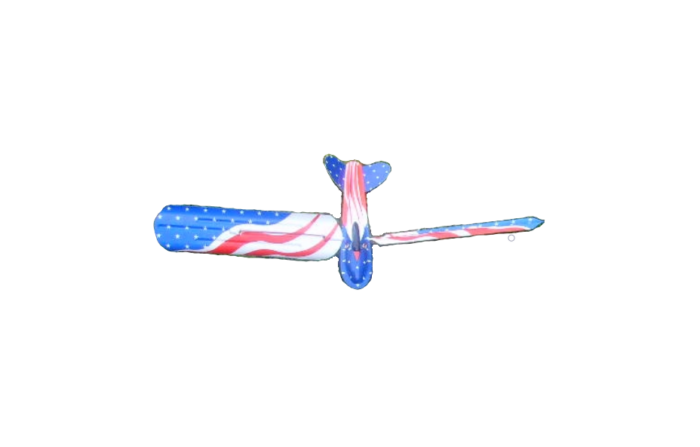
runcurvthikcamb.mwhich recovers the camber curve and thickness from an airfoil profile is given in .../Ch2 with some explanation in ../Ch2/Ch2Docs. It calls on functions in.../Ch2/Ch2lib. Run it on a few nacaxxxx profiles and check the statements about location of max thickness and camber. - Look up “Rotor Plane Kite”, a toy which uses rotating wings to create lift. Use the Kutta-Zhukowsky formula Eq. 2.5 to explain how it works. Quantitative results are probably hard to obtain, but you can try your hand on the “Flettner Rotor” propulsion for maritime applications. Google the FanWing/EU SOAR for an RC free-flight model.
- Assume a steady, inviscid, and incompressible flow. Show that
ρ|u|2/ R en + grad ρ = 0 ,
the streamline curvature equation, where en is the unit normal to the streamline x(t), dx/dt = u, and R is its radius of curvature. - Show that a potential flow satisfies the Euler equations, i.e. that there is a gradient which cancels the material velocity derivative.

